Time Series Meets Batch Macros
Time is a crucial aspect that must be addressed in our models, whether we are predicting the trend in financial markets or electricity use. For example, it would be useful to estimate when the peak demand of electricity will occur during the day to modify the price or output of electricity. Time series analysis is a specific way of analyzing a sequence of data points collected over an interval of time.
Many time series care only about the sum of all demand, or all sales. However, other use cases need to predict individual behavior – per customer – so that tailored incentives can be offered. (For example, offering a bonus only if the purchases exceed what they would have likely bought without the incentive.) For that, you can build a macro that carries out the processes repeatedly.
What makes a time series?
Any data that can be tracked and collected over time!
- Over a continuous time interval
- Of sequential measurements across the time interval
- Using equal spacing between every two measurements
- Each time unit having at most one data point
Time Series Analysis in Alteryx
Alteryx comes pre-loaded with seven time series tools. We can use these tools to study and analyze a time series before creating a forecast model. For the purposes of this blog, we will go over several of them in more detail.
There are two types of models that Alteryx offers: ARIMA and ETS. ARIMA uses an autoregressive integrated moving average and ETS uses an exponential smoothing method.
- Make sure there is no missing data prior to analysis – Of course data is not perfect and there may be instances in which you may have some empty periods. Ideally, you would want all periods filled to get the most accurate prediction of future data
- Run both models next to each other to see which has lower error – This is done by using the Alteryx tool TS Compare.
- TS Compare evaluates one or more time series created using either the ARIMA or ETS tools
- Build the model with a TS Forecast
- TS Forecast generates forecasts for a set number of future periods from an ARIMA or ETS model
The Use Case
You are working for a major airline company, and you want to evaluate the frequent travelers’ part of your proprietary traveler program. You want to provide incentives for your most profitable travelers to reach specific thresholds tailored to each individual. You need to start this analysis by predicting the next three months of airline miles for some of the airline’s highest frequent travelers.
The first step is to gather three years’ worth of data per traveler per month. How did I come up with three years? You want as much of a sample size as possible for the time series model to provide an accurate prediction.
The first part of this effort is to prepare the travelers’ data for it to be sent into a time series model. The data is organized in a horizontal fashion like the screen capture below.
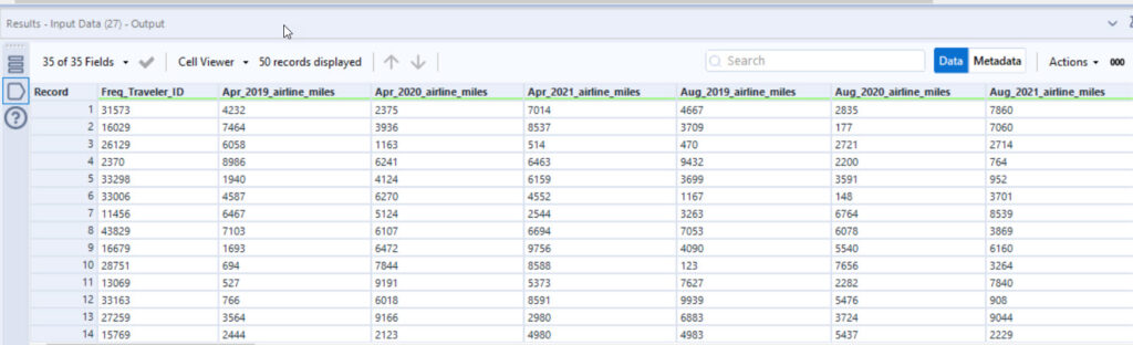
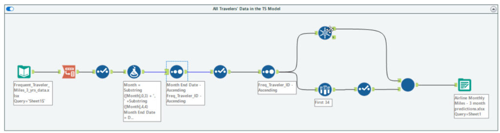
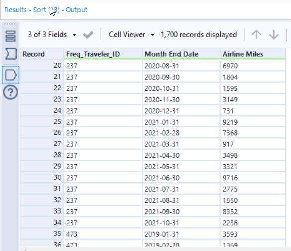
We need to transpose this data so that the time series model can accept the data. After we transpose the data, we separate the data by month and attach a month end date to each entry.
Now that data is organized properly, we need to send each traveler’s data into the time series model. To do that, we need to create a batch macro that would perform the time series analysis to predict the next three months of mileage output per traveler.
So, if your last collection of data is from Oct 2021, the next three months’ worth of data would be Nov 2021, Dec 2021, and Jan 2022. Let’s look at part of the batch macro that handles this.
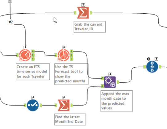
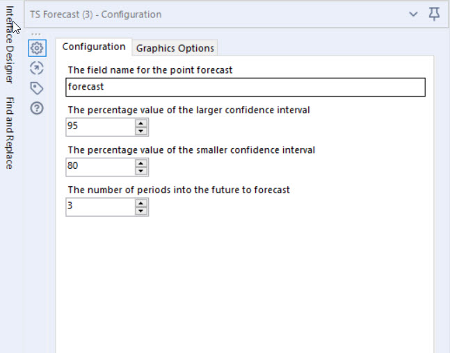
This portion of the macro illustrates how a single traveler’s data is sent to the ETS model. From there, the TS Forecast tool is used to predict the three months of mileage data. Configuring the TS Forecast tool is very simple. You provide a name for the forecast. I kept it simple by just calling it forecast. Then, you need to decide the confidence bounds you want to show, and the number of periods to create a forecast for. I wanted to have a large and small confidence interval, so I left the default values of 95 and 80 percent, respectively. Since we are looking to predict three months, I selected 3 for the periods. This will result in four fields being created: Forecast_High_95, Forecast_High_80, Forecast_Low_95, and Forecast_Low_80.
The top stream takes the Traveler ID. The second stream gathers the predicted monthly airline miles. The lower stream finds the latest month end date of data. That gets appended to the predicted values and, eventually, appended to the Traveler ID.
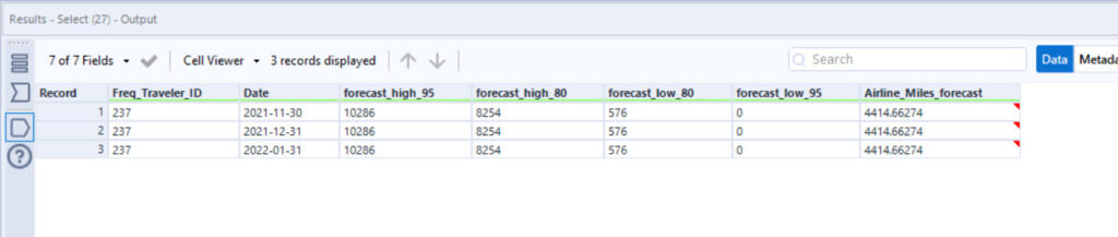
When the macro is completed, three rows of data with the following fields are returned to the primary workflow: Traveler ID, Predicted Date, Forecast_High_95, Forecast_High_80, Forecast_Low_95, Forecast_Low_80, Airline Miles Forecast.
Performing time series can be a labor intensive within Alteryx because R is opened for every frequent traveler in your dataset. Leave some time and some space on your hard drive to execute a large dataset of travelers or any other use case that you might find that is like this one.